library(tidyverse)
library(brms)Visualize and select priors
To get started, we load the required packages.
Selecting Priors
A prior distribution in Bayesian analysis will assign a probability to each possible value of a parameter. By specifying priors, brms takes into account not only the inputted data but also what is already known about the likelihood of certain parameter values to produce a more accurate estimation.
Confusion of whether prior applies only to intercept or also to between-group coefficients
Trying to make prior on eta be specific to the Intercept, eta_Intercept
From brms documentation: In case of the default intercept parameterization (discussed in the ‘Details’ section of brmsformula), general priors on class “b” will not affect the intercept. Instead, the intercept has its own parameter class named “Intercept” and priors can thus be specified via set_prior(“
In an attempt to get eta_Intercept instead of Intercept_eta, that my changing class from “b” to “Intercept” did, try also specifying coef.
Wow, specifying both class as “b” and coef as “Intercept” resulted in “Intercept_eta_Intercept” inside brms!
Error : The following priors do not correspond to any model parameter: <lower=0,upper=2.5> Intercept_eta_Intercept ~ uniform(0, 2.5)
So try leaving class blank while keeping coef=“Intercept”, as that seems to be what puts “Intercept” before “eta”.
That results in this error: Error : Prior argument 'coef' may not be specified when using boundaries.
So I dropped lb and ub.
That yields a warning because the uniform prior I set does have bounds, and brms doesn’t like that discrepancy.
Warning :It appears as if you have specified a lower bounded prior on a parameter that has no natural lower bound. If this is really what you want, please specify argument 'lb' of 'set_prior' appropriately. Warning occurred for prior b_eta_Intercept ~ uniform(0, 2.5)
Final solution for an eta uniform prior only on the Intercept:
#brms can't evaluate parameters in the prior setting so one has to resort to sprintf-ing a string, if you want to set parameters dynamically
eta_param1<- 0
eta_param2<- 2.5
eta_prior_distribution<-  sprintf("uniform(%s, %s)", eta_param1, eta_param2)

brms::set_prior(eta_prior_distribution,
                   coef="Intercept",
                   nlpar = "eta")
b_eta_Intercept ~ uniform(0, 2.5)Prior on Lapse \((L)\)
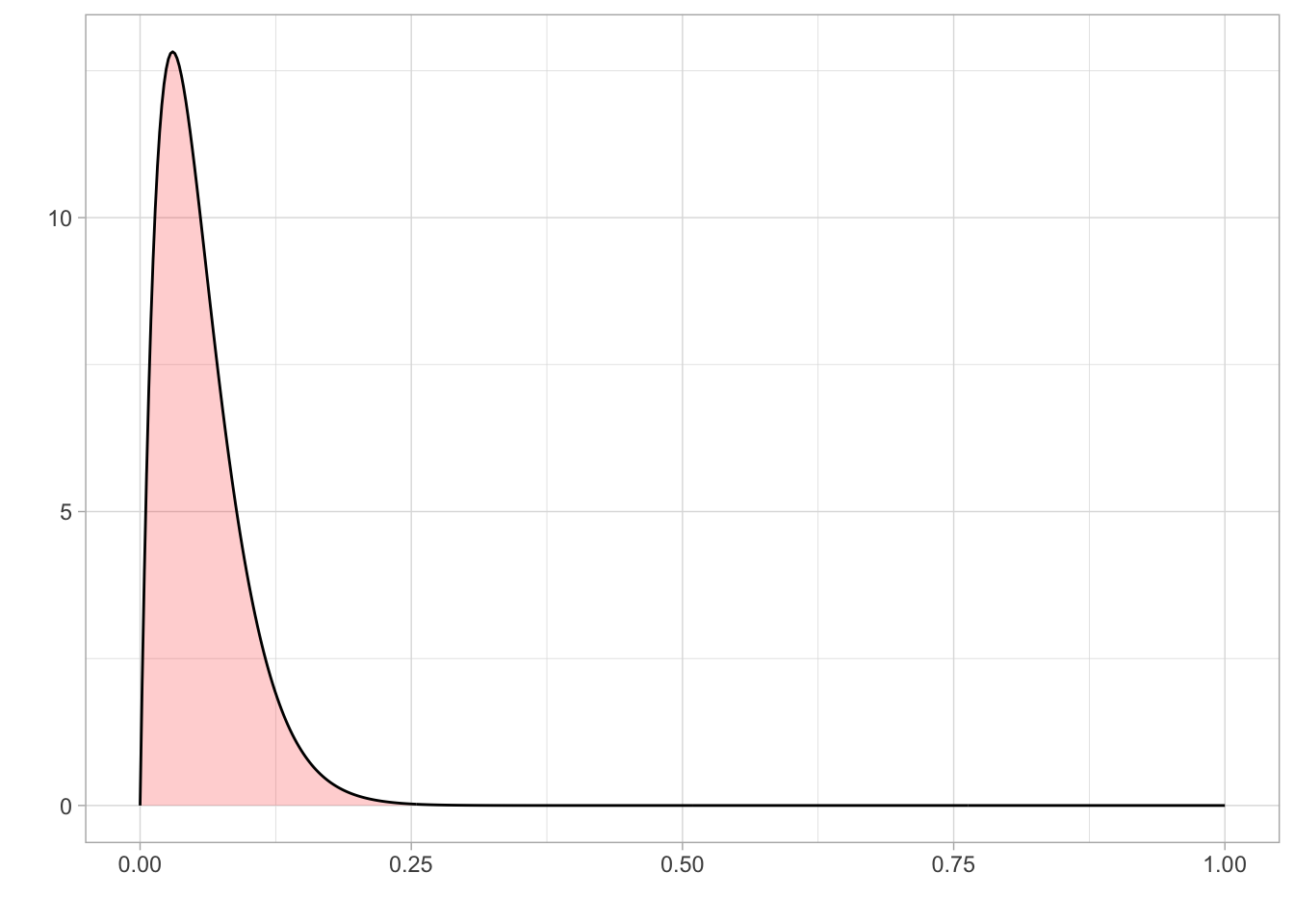
Since lapse is a rate, it is bounded between 0 and 1. We know from previous literature that a reasonable value of lapse is between 0.03 and 0.04.
As the tested population was reasonably well-motivated, high lapse valuables were unlikely, although not impossible. Therefore, we set a prior on lapse using a beta distribution that was bounded between 0 and 1 and a mode of 0.03.
lapse_param1<- 2
lapse_param2<- 33.33
prior_lapse <- dplyr::tibble(
x = seq(0, 1, length.out = 500),
y = dbeta(x, lapse_param1, lapse_param2)
)
ggplot(prior_lapse) + aes(x = x, y = y) +
geom_area(fill = "red", alpha = 0.2) +
geom_line()+
theme_light() +
labs(
x = "",
y = ""
)
Prior on Location \((\eta)\)
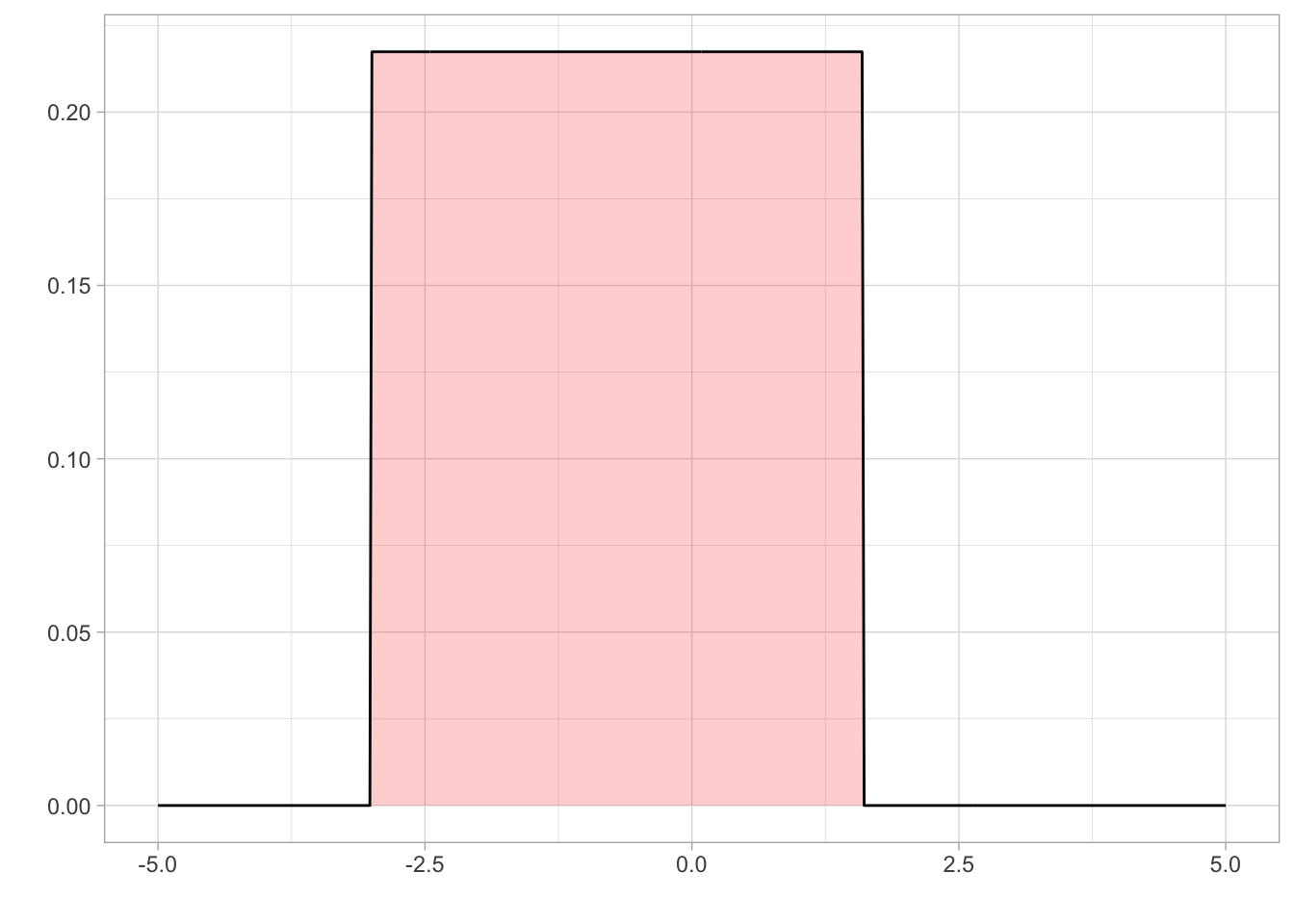
We set a uniform prior for location with a lower bound of 0 and an upper bound of 2.5. The lower bound was set at 0 as you cannot have negative speed . Holcombe and Chen (2013) found that even the best participant would have a speed threshold of less than 2.5 revolutions per second, even with only 2 distractors present in their array. Holcombe and Chen (2020) found that tracking of a single object on a mechanical display which is not confounded by a display’s refresh rate still had a speed limit of 2.3 revolutions per second. Therefore, from previous research, an upper bound on speed threshold at 2.5 revolutions per second would be adequate to cover all participants.
eta_param1<- 0
eta_param2<- 2.5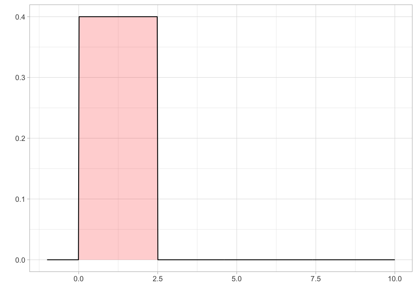
Prior on Sigma/Scale \((\sigma)\)
Values of sigma can get extremely small and therefore tiny changes in the value of sigma can have significant effects, makeing it hard for brms to accurately estimate sigma. Therefore, our brms model is cast in terms of logsigma. We concluded that a sigma approximately between 0.05 and 5 would be a sufficient range to accommodate all participants based on looking at psychometric data from previous papers. Converting this with the log transform, we set a uniform prior on logsigma with a conservative lower and upper bound of -3 and 1.6 respectively.
logsigma_param1<- -3
logsigma_param2<- 1.6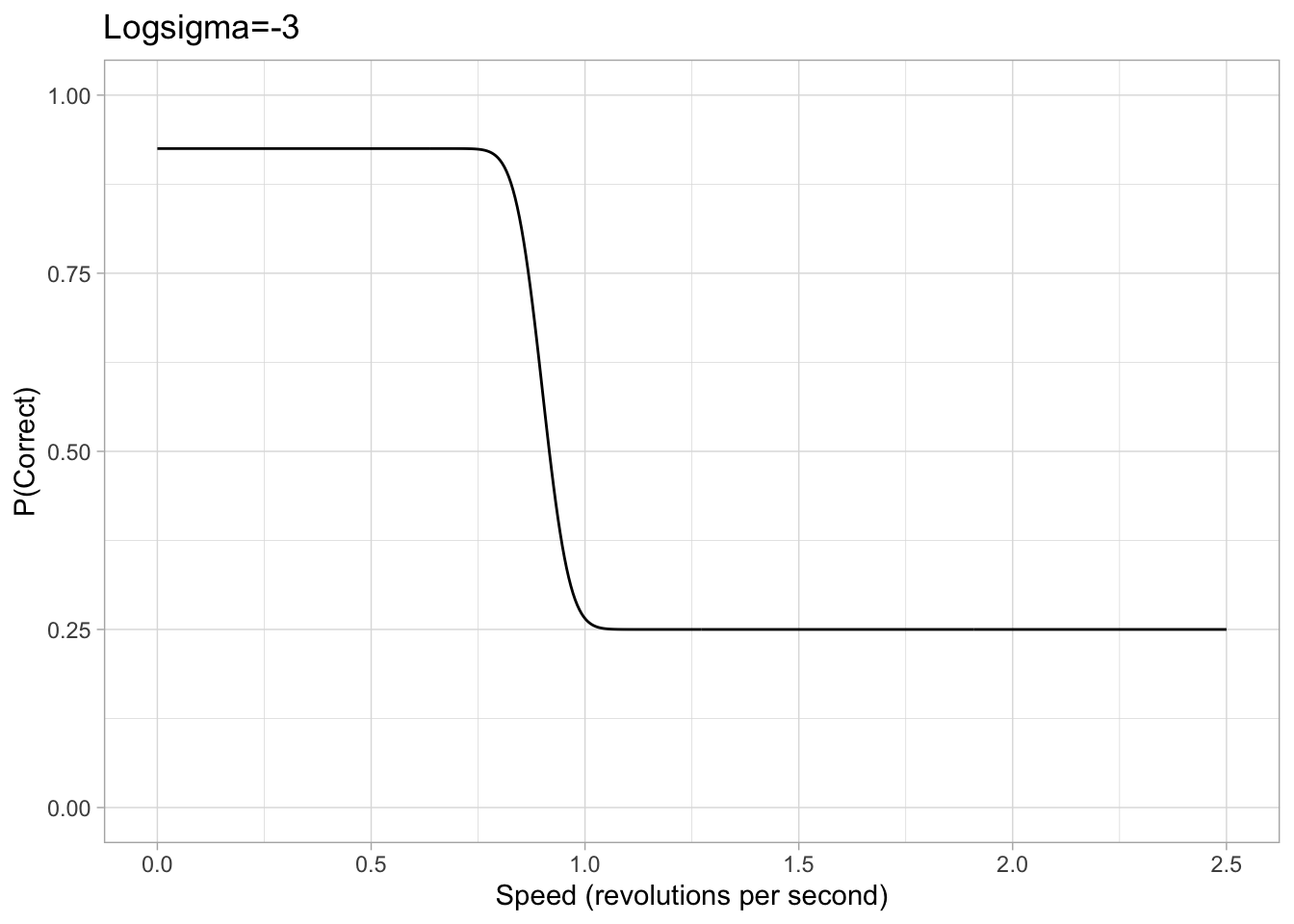
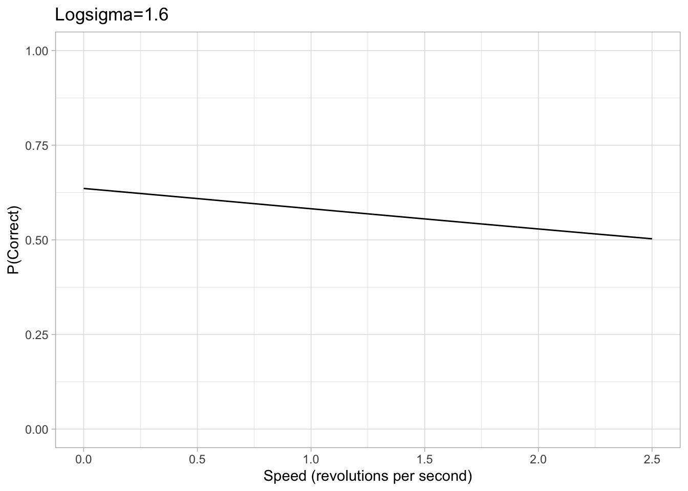
Figure 2: Example plots of psychometric function with a logsigma of either -3 or 1.6. The chance rate, eta and lapse are all consistent with the previous example.
Plot them all together
Warning: Removed 373 rows containing missing values or values outside the scale range
(`geom_line()`).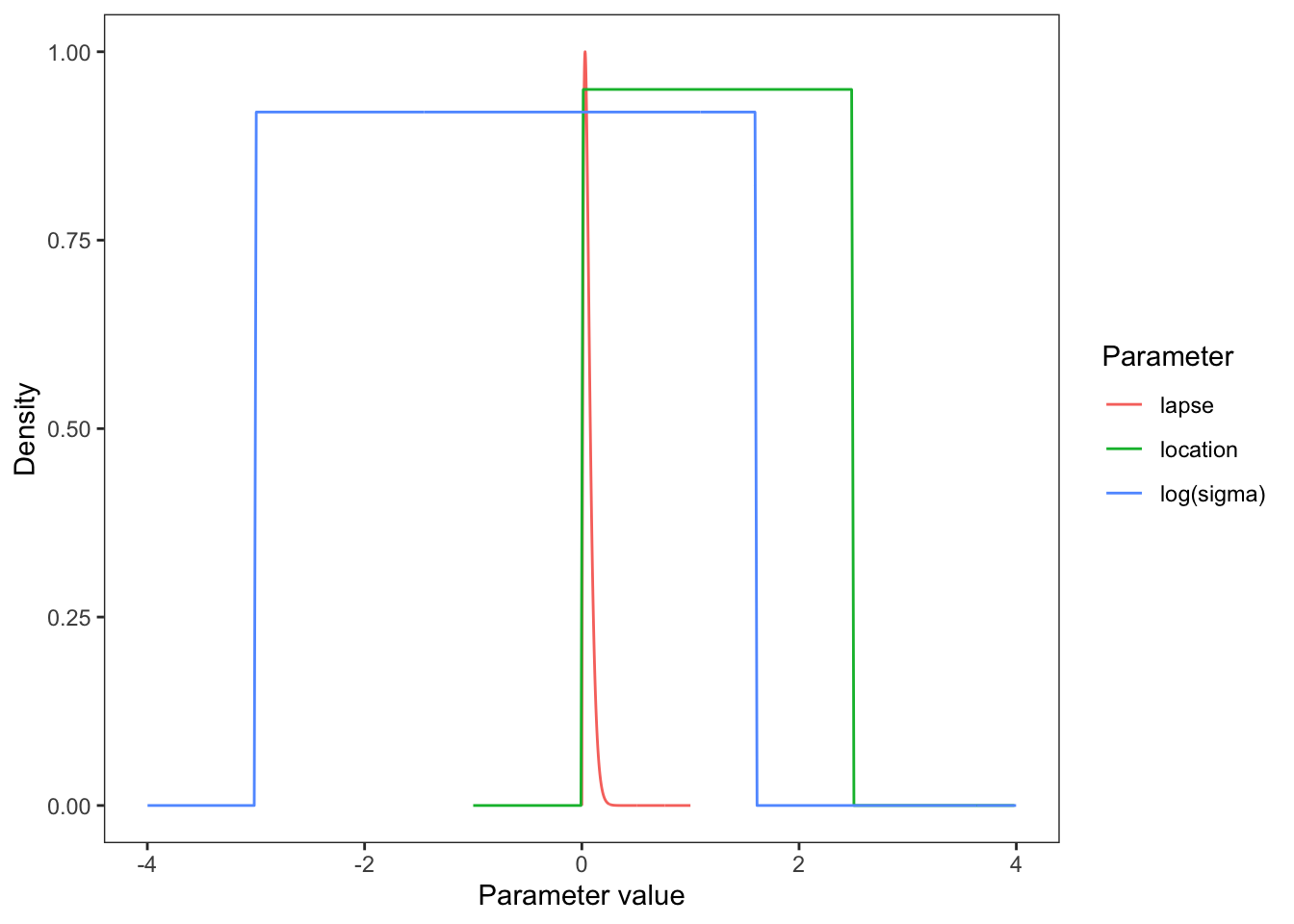
Here is code you can use when calling brms:
#brms can't evaluate parameters in the prior setting so one has to resort to sprintf-ing a string
# if you want to set the parameters dynamically
lapseRate_prior_distribution<- sprintf("beta(%s, %s)", lapse_param1, lapse_param2)
eta_prior_distribution<-  sprintf("uniform(%s, %s)", eta_param1, eta_param2)
logsigma_prior_distribution<- sprintf("uniform(%s, %s)", logsigma_param1, logsigma_param2)

my_priors <- c(
   brms::set_prior(lapseRate_prior_distribution, class = "b", nlpar = "lapseRate", lb = 0, ub = 1),
   brms::set_prior(eta_prior_distribution, # class = "Intercept",
                   coef="Intercept",
                   nlpar = "eta"),#, lb = 0, ub = 2.5),
   brms::set_prior(logsigma_prior_distribution, class = "b", nlpar = "logSigma", lb = -2, ub = 1.6)
 )